Rendering with Indigo
This section begins with a simple overview of rendering with Indigo, followed by sections for various features and settings used for rendering.
Comprehensive coverage of Indigo's material system can be found in the "Materials" section.
Render Tutorial
In this tutorial we will render an example scene that comes with Indigo to illustrate the basic render settings.
-
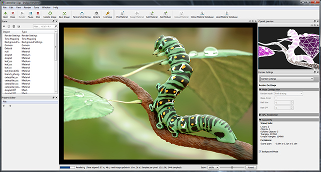
Start Indigo and click the Open button in the toolbar. Browse to the "testscenes" subdirectory in your Indigo Renderer installation, which on Windows is usually C:\Program Files\Indigo Renderer\testscenes.
Open the "Caterpillar" example; this scene, by Paha Shabanov, showcases a number of Indigo's more complex features (e.g. displacement, subsurface scattering) and won a competition held on our Forum to be included with the Indigo distribution. -
This scene renders quite slowly using the default Bi-directional Path Tracing render mode, so let's set it to use the simpler, non-Bi-directional (i.e. single-directional) path tracing mode.
In the Render Settings view (on the right side of the image), from the drop-down menu at the top, select the "Render Settings". From the "Render mode" drop-down, select "Path tracing". -
Now we're ready to begin rendering. Hit the "Render" button on the toolbar, and Indigo will begin "building" the scene (preparing it for rendering).
For simple scenes, this build process will be nearly instantaneous, but for larger scenes (with many polygons, subdivision surfaces etc.), building the scene can take a little while. Indigo displays the build progress in the status bar, and you can see the full log by clicking the "Render Log" drop-down option from the Render Settings view. -
Once the scene has started rendering, the status bar will continually update with information about the render in progress.
Particularly relevant is the number of samples per pixel, which can be roughly thought of as the image quality; every so often (with decreasing frequency) the image will automatically update as it's rendering. You can update the image at any time either via the Update Image toolbar button or by pressing F5. -
After some minutes of rendering the "noise" (or graininess) in the image will go away, leaving a nice clean render:
-
Next we'll illustrate some of the imaging settings; these affect the appearance of the final image from the physical light computation Indigo performs, and can be adjusted without restarting the render.
In the Render Settings view, select "Imaging" from the drop-down at the top. The default setting for this scene is Camera tone mapping with the FP2900Z preset, and we can change its exposure (EV) and film ISO as with a real camera. If we switch the method to "Reinhard", Prescale to 2 and Burn to 3.6, we get the following result with less saturation, but also less "blow out" in the bright regions:
-
In the White Point section we see that the scene's default white point is the "E" preset. Typically we use a D65 ("daylight") white point, and selecting this option produces a noticeably "warmer" image:

-
Finally, let's save this image to disk; click the "Save Image" button in the toolbar, and either give the image a new file name or leave it as is.
Saving as PNG is generally recommended instead of JPEG unless the image will be directly uploaded to the Internet and needs to be compressed, since every time a JPEG image is saved the image quality is reduced (as it is a "lossy" format, as opposed to PNG which is "lossless" i.e. a perfect copy).
Denoising
Since Indigo 4.4.1 beta, Indigo has integrated Intel's Open Image Denoise.
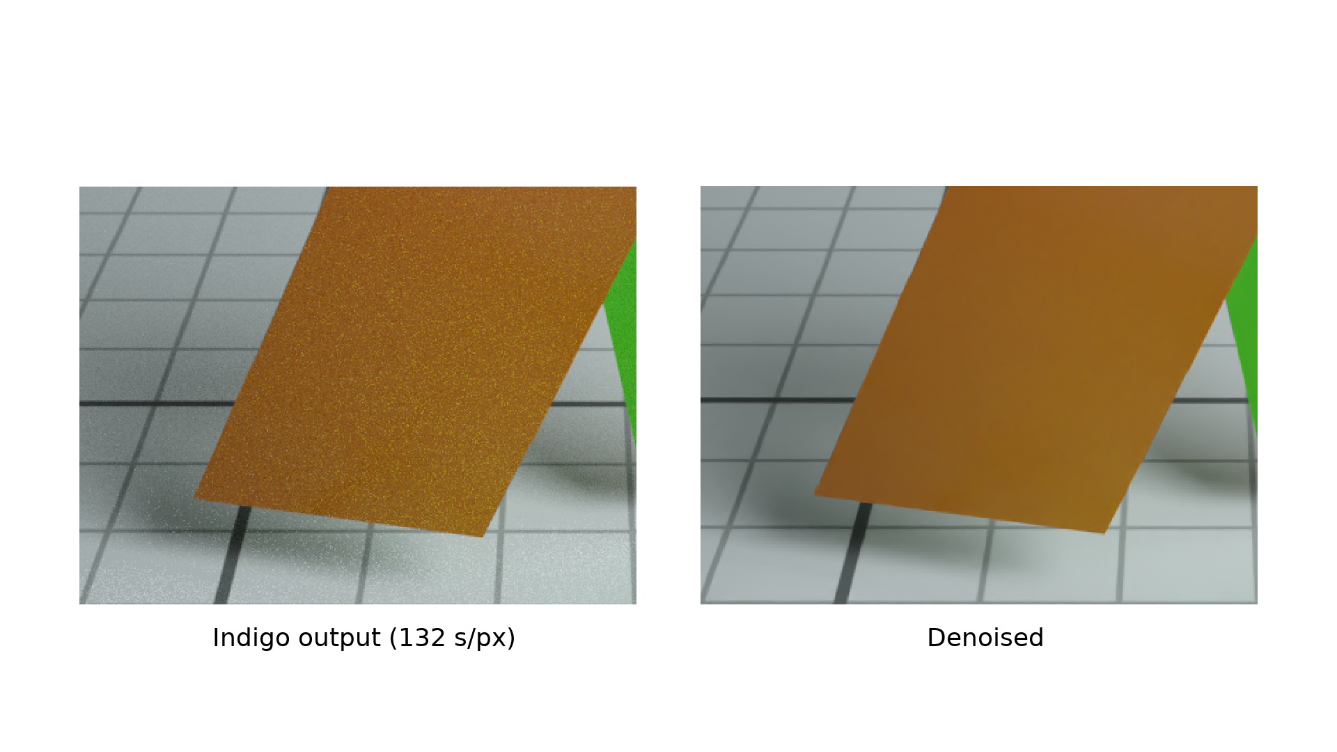
Optimising for denoising
The denoiser requires some additional information to work at maximum effectiveness - in particular it requires the normals and albedo render channels to be enabled.
This can easily be accomplished by checking the 'Optimise for Denoising' checkbox:
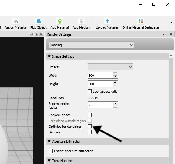
Checking or unchecking this checkbox will restart the render.
Enabling or Disabling denoising
Denoising can be enabled or disabled during rendering with the 'Denoise' checkbox. Checking or unchecking this checkbox won't restart the render.

Denoising is computed each time the image is updated and displayed.
Denoising takes some time to compute - especially for high resolution images, and high supersampling factors.
If it is taking too long, try reducing the supersampling factor (for example to 2 or 1).
More denoising examples
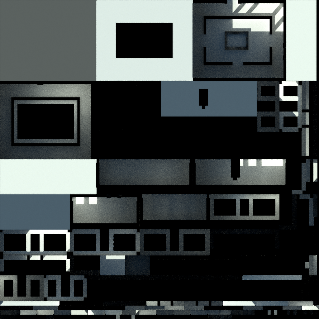
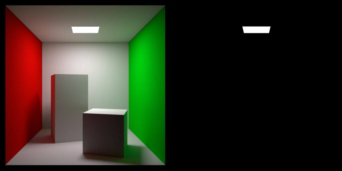
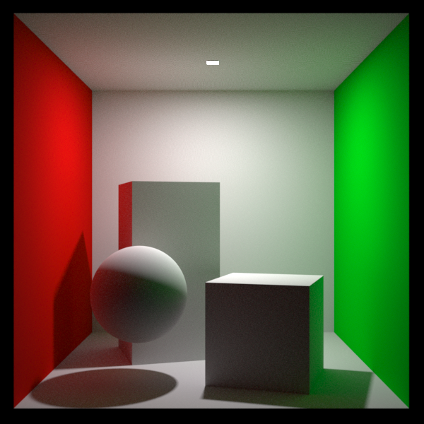
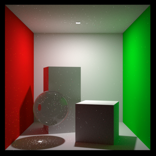
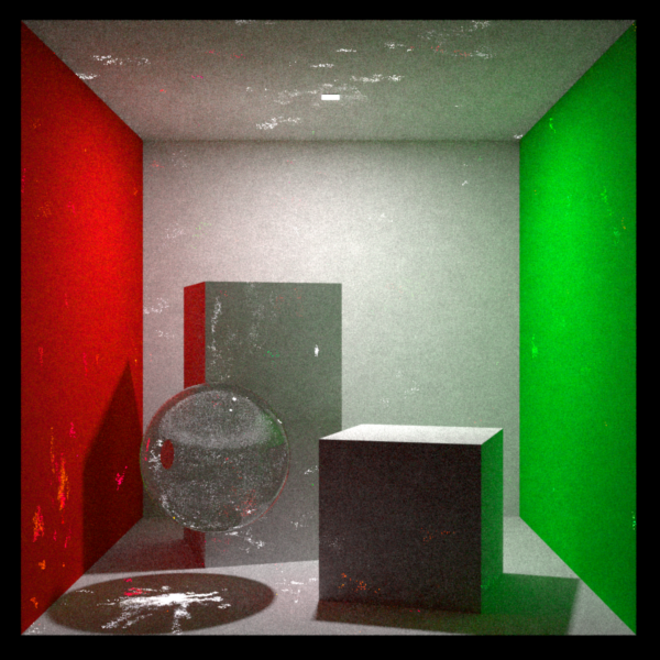
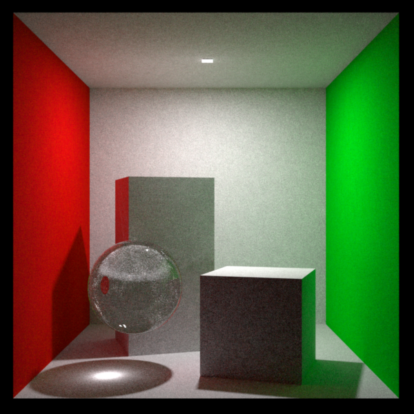
A render without denoising. The room scene by Lal-O is included in the Indigo distributon.

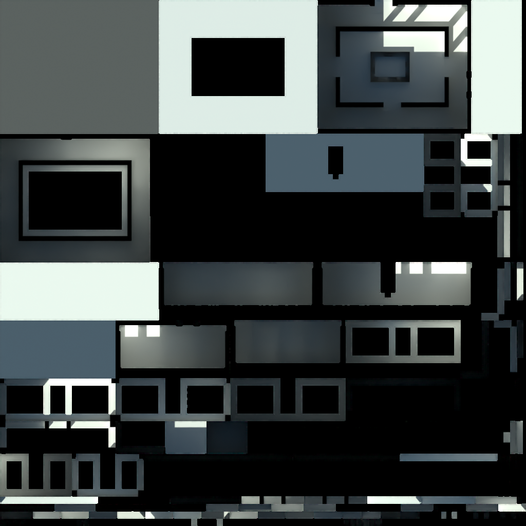
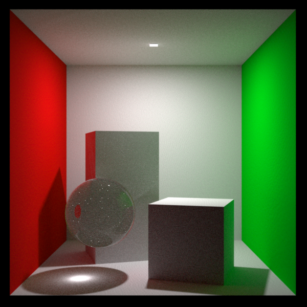
The render with denoising.
Environment Settings
There are several options that allow you to define the appearance of empty space around your scene. This listing is not exhaustive, since any material can be used as the background material, however we'll most list the commonly used settings here.
Constant colour background

Illuminates scene with a uniform environment light.
Sun & sky
Indigo comes with a Sun and Sky environment that realistically depicts the sky. Changing the sun's direction creates time-of-day effects: a low angle creates a sunrise/sunset with correctly coloured sky and brightness.

The classic Sun & Sky model.
The following options are available for the classic model:
Turbidity: The turbidity defines the haziness/clearness of the sky. Lower turbidity means a clearer sky. Should be set to something between 2 and ~5.
Extra Atmospheric: Removes the sky and renders only the sun. Good for renders in space.
Since Indigo 3.2, there is also a new "captured" sky model, which is actually simulated by Indigo and captured to disk with the distribution.

The captured Sun & Sky model.
Environment map

Illuminates scene with an environment map, which usually is a high dynamic range (HDR) image.
Indigo can load HDR environment maps in three formats, EXR (file extension .exr), RGBE (file extension .hdr) and a raw data format (extension .float, a simple format exported by the HDR Shop program); the environment map must either be in spherical format or equarectangular.
There are a number of setting available currently for environment maps. The emission values should usually be quite high, approximately 10^7 to be similar to the sun's brightness. The "Advanced Mode" checkbox ticked gives the users more options (full control over the image including Gamma and Texture Mapping modes), while disabling it reveals easy to use controls for rotating and tinting the environment map.
GPU Rendering Guide
GPU drivers
The first and most important point is: you must update your GPU drivers.
GPU compute depends very strongly on the quality of GPU drivers, and the various GPU manufacturers have been doing a great job of updating their drivers to be faster and more robust.
NVIDIA driver downloads: http://www.nvidia.com/drivers
AMD driver downloads: http://support.amd.com/en-us/download
Intel driver downloads: https://downloadcenter.intel.com/
Recommended GPU specifications
NVIDIA
GTX 660 Ti or better
Quadro K4000 or better
AMD
Radeon HD 7770 or better
FirePro W5000 or better
Older graphics cards might work with OpenCL rendering, but may cause problems and are unlikely to provide any significant performance gain compared to Indigo's highly optimised CPU rendering.
Memory limitations
One of the major limitations for GPU-based rendering is the amount of onboard memory available, which is typically 2-4 GB for desktop GPUs, while CPUs can easily have 32 GB. Because of this, you might run out of memory when trying to render scenes with lots of geometry and high resolution textures.
The Max Individual Allocation reported by Indigo is the largest amount of memory that can be allocated at once with OpenCL, e.g. for textures. Indigo performs multiple allocations for every scene. The practical limitation at this point is that the total texture size is limited to 25% of total GPU memory on NVIDIA, and about 65% of total GPU memory on AMD.
Using the computer while rendering
A well-known side effect of using your primary GPUs (ones which are connected to a display) while rendering is that your operating system can lag quite substantially. The best way around this is to have a GPU dedicated for display (usually a small inexpensive card, or perhaps the integrated GPU of some CPUs), while the others are dedicated for rendering. This also helps to reduce the memory overhead, which can be important in GPUs with <= 2 GB of memory running high resolution desktop and lots of web browser tabs etc.
Kernel compilation
Indigo uses a combination of OpenCL and our own programming language, Winter, for the rendering core. This means that when you start rendering a scene, the GPU drivers must compile the OpenCL code, and this process can take some time, depending on the complexity of the scene.
When using multiple GPUs, the kernel builds for each GPU are done in parallel to make better use of the CPU cores, however most GPU drivers do not do multi-core compiling themselves, so future driver updates could improve this without any changes in Indigo.
We are working on making kernel builds faster and less frequent.
Lightmap baking
Lightmap baking
Indigo 4.4.10 introduced a lightmap baking feature.
Lightmap baking is the rendering of a lightmap. A lightmap is an image map that represents the light (or in particular, the irradiance) at points on the surface of an object. Lightmaps are usually used for realtime 3d rendering, for example in computer games or VR experiences.
Lightmap baking in Indigo allows a lightmap to be computed with full unbiased physically-based spectral rendering with global illumination.
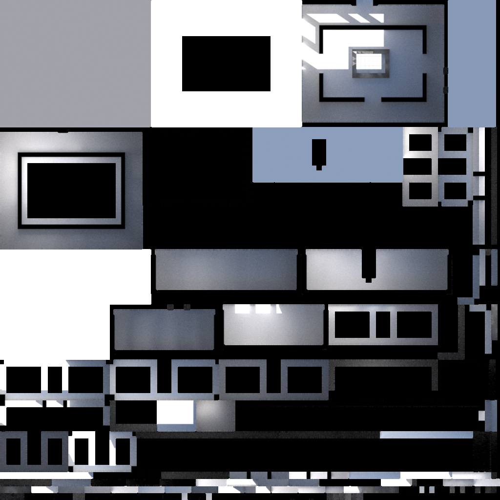
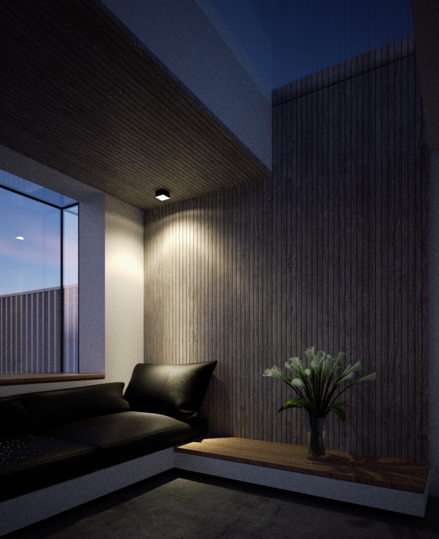
A lightmap baked in Indigo

The lightmap used in a realtime OpenGL 3d engine.
UV unwrapping
Lightmaps require a special UV mapping, generally in which each piece of geometry appears just one in the UV map, and there are no overlaps. The process of generating such a UV map is called UV unwrapping.
Indigo can optionally perform this UV unwrapping process, or it can use an existing UV mapping present in the mesh data.
How to use lightmap baking in Indigo
To perform lightmap baking with Indigo, you will need to either enable lightmap baking in the render settings user interface, or alternatively edit your scene file.
To enable in the user interface, select an object in the 'Object to bake' box:
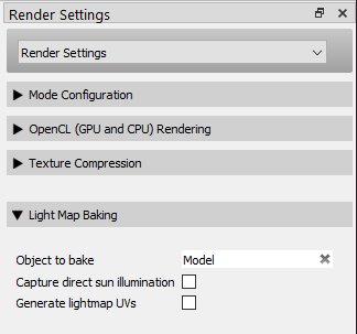
You should check 'Generate lightmap UVs' unless you know your object mesh already has a suitable UV map.
You can alternatively edit your scene file (.igs file, which is just XML), and set the following render settings in your <renderer_settings> element: (see https://www.indigorenderer.com/indigo-technical-reference/indigo-scene-f...)
light_map_baking_ob_uid
If set to a valid UID (>= 0), Indigo will compute a lightmap for the object with the given UID.
type: int
default value: -1
generate_lightmap_uvs
If set to true, Indigo will generate a UV mapping for the mesh that it is computing lightmaps for, if any (see light_map_baking_ob_uid). The new UV mapping will be added to the mesh after the existing UV mappings.
For example, if the mesh has a single UV mapping with index 0, then a new UV mapping will be created with index 1.
The modified mesh with the additional UV mapping will be saved to disk at 'mesh_with_lightmap_uvs.igmesh' in the Indigo Renderer application data dir. (e.g. C:\Users\xx\AppData\Roaming\Indigo Renderer)
If generate_lightmap_uvs is false, then the UV mapping with the highest index in the mesh will be used as the lightmap UV mapping.
type: boolean
default value: false
capture_direct_sun_illum
This option only has an effect when computing a lightmap.
If set to false, direct illumination from the sun will not be captured in the light map. This is useful in the case that direct sun illumination will be rendered using some other technique at runtime, for example shadow mapping.
type: boolean
default value: true
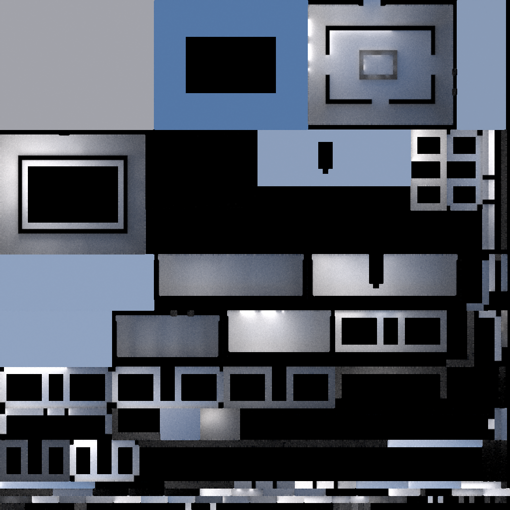
A lightmap with capture_direct_sun_illum set to false; compare with the lightmap above.
Saving your lightmap
Indigo renders lightmaps much like usual renders with a simulated camera. As such you can save the lightmap in the standard ways, including with the Save Image toolbar button, which saves tonemapped, LDR image. You can also save out a HDR un-tonemapped EXR, with the Render > Save un-tonemapped image command.
Denoising
Indigo's integrated denoiser also works very effectively with lightmaps. You can enable denoising by checking the 'Denoise' button in the Image Settings controls in the Render Settings area.
Lightmap without denoising
Lightmap with denoising (same render time)
Object Settings
There are some settings that apply to individual objects. (sometimes referred to as instances)
Please read on for details.
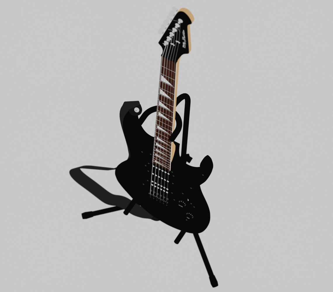
Invisible to Camera
The invisible to camera option makes an object invisible to the camera, at least as seen directly.
However, the object will still cast shadows, and will be visible in reflections from other objects.
The invisible to camera option is useful in a few different scenarios:
- Hiding a wall in an architectural rendering so there is more space for the camera.
- Hiding an object when doing a shadow pass, so that the object does not get in the way of the shadows cast on the ground. See the Compositing with shadow pass tutorial for more information.
- Hiding a light source, where the light source would usually be visible in the 'shot'.

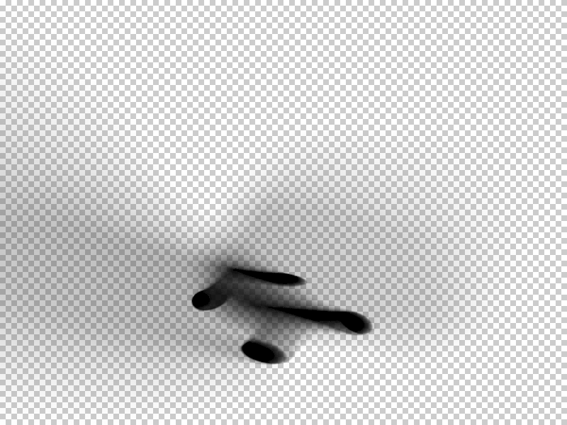
Piggy bank with piggy visible to the camera
Piggy bank with piggy invisible to the camera. Note that shadows from the piggy are still present.
Setting to invisible in the Indigo GUI
To make an object invisible to the camera in the Indigo user interface, first select the object with the pick object tool:

Then check the invisible to camera checkbox in the Property Editor:
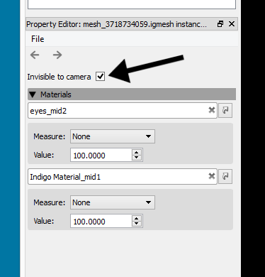
The invisible to camera option is in Indigo Renderer only and is not available in Indigo RT.
Region rendering
Region rendering allows you to render only a small part of the scene. This is similar to moving the camera, but is useful when you need to focus the render on a part of the full image.
As of version 4, Indigo lets you render multiple regions sequentially and/or simultaneously. There is also an option to either render the region(s) on top of the full image buffer, or on an alpha background outside the regions for compositing in post production software.
Using render regions
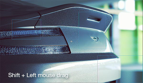
To use region rendering, simply enable the "Pick Region" button from the tool bar. This will enable Region Render under Imaging settings, and will let you select your region by using LMB + drag. To render multiple regions at once, hold Shift or Ctrl and drag.

To render your regions on an alpha background, enable the "Zero alpha outside region" checkbox below the Region Render one. This option can be enabled and disabled without re-rendering.
Unchecking the Region Render checkbox will disable region rendering and render the full image buffer. Rechecking Region Render will use your previously used region(s). Camera movement will also disable region rendering for easier maneuvering.
Multiple regions

Zero alpha outside region
Render Channels
Render channels allow extra information to be rendered from the scene.
Beauty render channels are components of the final 'beauty' render, where each render channel captures all the light from a particular class of path from the emitter to the camera.
Non-beauty render channels allow additional information (usually geometric information) to be generated, such as depth, normals, position, or material and object masks.
Support for Render Channels
Render channel support was introduced in Indigo Renderer 4.2.
Render channel support is available in Indigo Renderer, but not in Indigo RT.
Enabling Render Channels
Render channels can be enabled or disabled in the Render Channels page in the Render Settings widget:
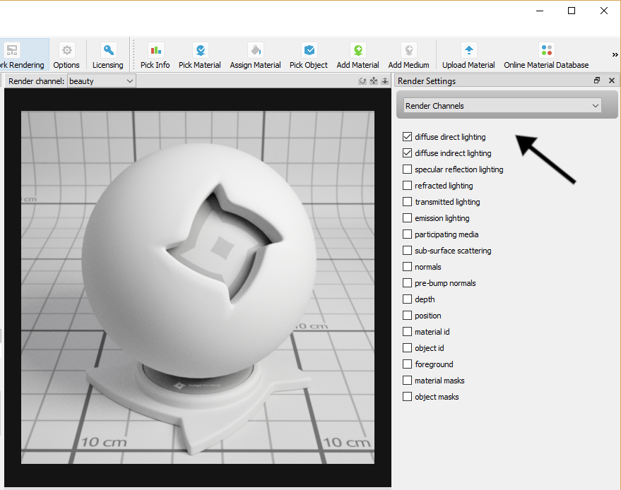
Render channel settings.
Note that enabling or disabling a channel will restart the render if it is rendering.
Viewing Render Channels
To change which render channel is shown in the Indigo user interface, you can use the drop-down box above the render display:
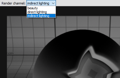
Select render channel to display.
Only enabled render channels will be available in the drop-down box.
Saving Render Channels
You can save the render channels to disk with the Save Layers and Channels menu command in the Render menu.
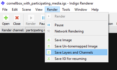
Save Layers and Channels Menu command.
Combine into single file option
This option can be found in the Indigo Options dialog (Tools > Options), in the Image Saving tab.
If enabled, all light layers and enabled render channels are combined into a single EXR file when saving with the Save Layers and Channels menu command.
If disabled, then one EXR file is saved for each light layer and for each enabled render channel. The filenames will have the channel name as a suffix, for example render_channel_test_depth.exr, render_channel_test_normals.exr etc..
Beauty Render Channels
Beauty render channels are components of the final 'beauty' render, where each render channel captures all the light from a particular class of light path from the emitter to the camera.
Direct Lighting Channel
This render channel shows direct diffuse lighting.
In other words, it shows light that is emitted from a light source, and then bounces exactly once diffusely off an object
and into the camera.
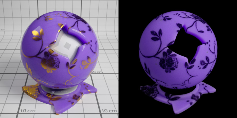
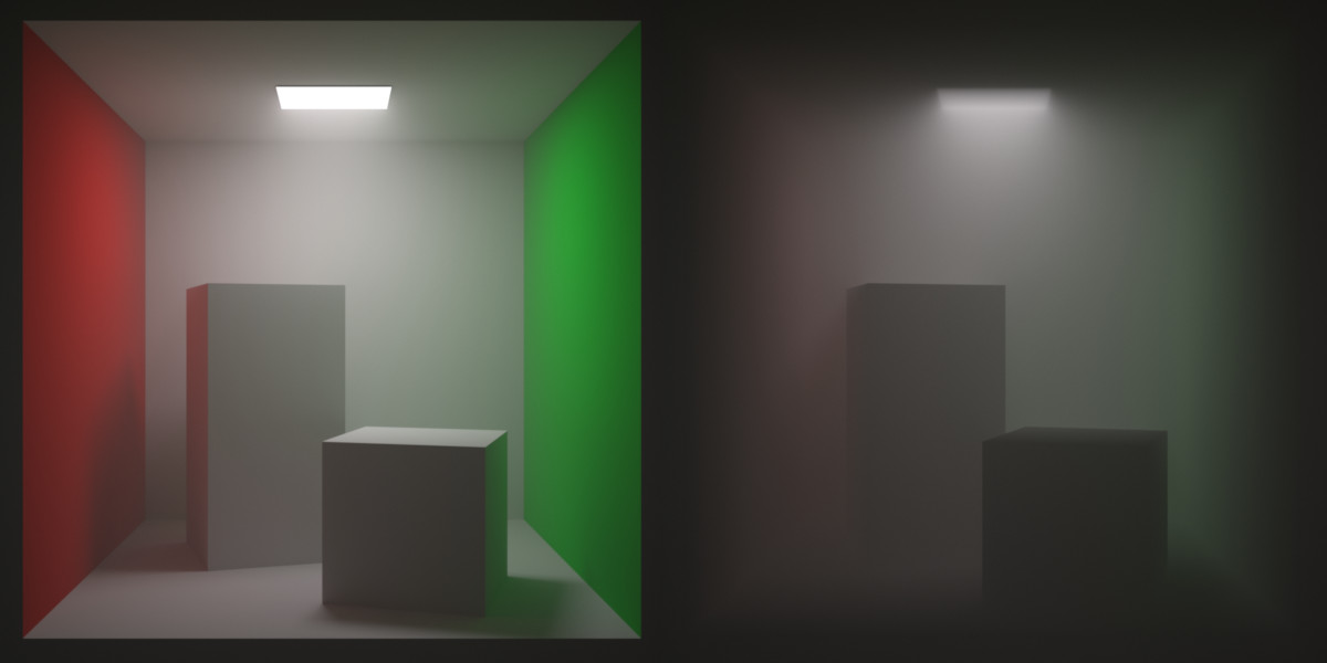
left image - beauty render. right image - direct lighting channel
Indirect Lighting Channel
This render channel shows indirect diffuse lighting.
In other words, it shows light that bounces around a scene at least once, and then bounces diffusely off an object immediately before hitting the camera.
left image - beauty render. right image - indirect lighting channel
Specular Reflection Lighting Channel
This render channel shows specularly reflected light.
In other words, it shows light that bounces around a scene, and then bounces specularly (e.g. bounces off a smooth surface) off an object immediately before hitting the camera.

right image - Specular reflection channel
Refracted Lighting Channel
This render channel shows refracted light.
In other words, it shows light that bounces around a scene, and then is refracted through a transparent object immediately before hitting the camera.
Glossy transparent and specular materials will contribute to this channel.
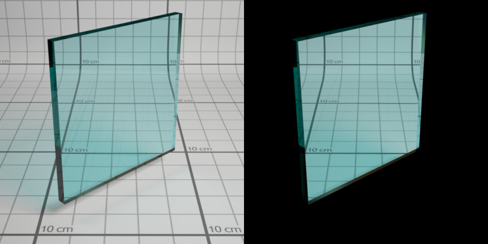
right image - refracted lighting channel
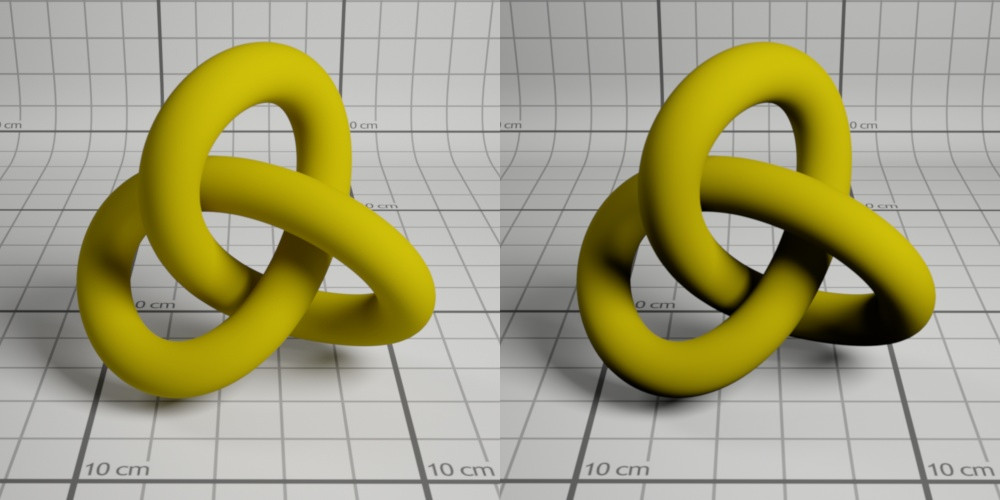
Transmitted Lighting Channel
This render channel shows light diffusely transmitted through a surface.
In other words, it shows light that bounces around a scene, and then is diffusely transmitted through a partially or full transparent object immediately before hitting the camera.
Diffuse transmitter and double-sided thin materials will contribute to this channel.
A double-sided thin material. Right image - transmitted lighting channel
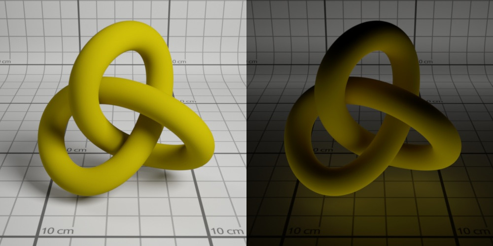
Emission Lighting Channel
This render channel shows directly emitted light.
In other words, it shows light that is emitted from a light source, and then directly strikes the camera.
right image - emission lighting channel
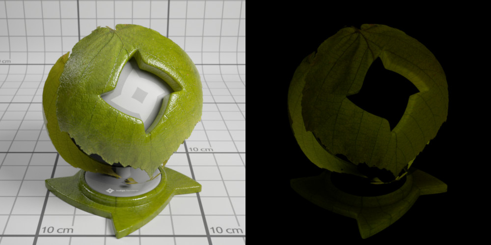
SSS Lighting Channel
This render channel shows light that has undergone sub-surface scattering.
In detail - it shows light that is emitted from a light source, bounces around the scene,
undergoes SSS, exits a medium through a transparent material, and then directly strikes the camera.
right image - SSS lighting channel
Participating Media Lighting Channel
This render channel shows light that has undergone participating-media scattering.
In detail - it shows light that is emitted from a light source, bounces around the scene,
undergoes participating media scattering, then directly strikes the camera.
right image - Participating Media lighting channel
Non-Beauty Render Channels
Normals Channel
This render channel shows the normalised surface normal in world space.
Channel values will range from -1 to 1.

Normals pre-bump Channel
This render channel shows the normalised surface normal in world space, before bump mapping was applied.
Channel values will range from -1 to 1.

Depth Channel
This render channel shows the distance from the camera to the first hit point along a ray from the camera, divided by the diameter of the scene.
Channel values will range from 0 to 1.

Position Channel
This render channel shows the world-space position of the surface.
Channel values have no fixed range and may be negative.

Material ID Channel
This render channel has a pseudo-random colour assigned to each material.

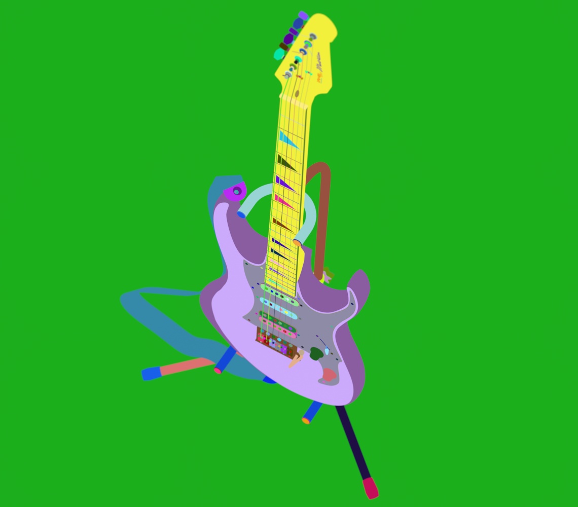
Object ID Channel
This render channel has a pseudo-random colour assigned to each object.
Albedo Channel
This render channel shows the albedo (colour) of the hit material. For specular materials the path is continued and the reflected or refracted albedo is shown instead.
In Indigo 4.4.1 or newer.
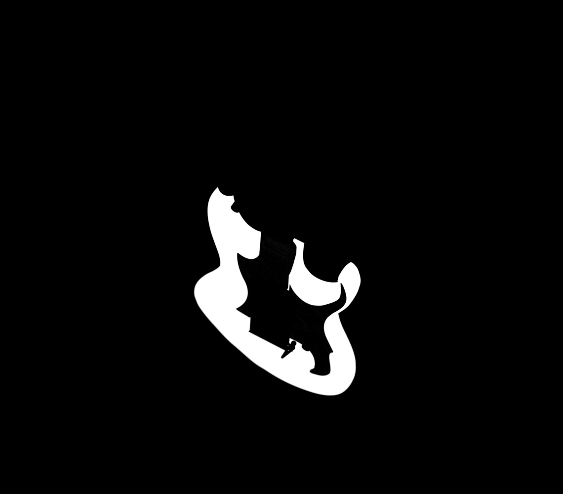
Material Mask Channels
You can have multiple material mask channels.
All materials that have a common mask name will be rendered white - everything else will be rendered black.
There will be a material mask channel automatically created for each unique material mask name set in the scene.
Don't forget to enable the material masks checkbox in the Render Channels tab to turn on the material mask channels!

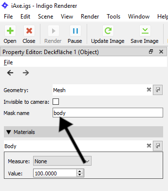
You can set the material mask name in the Indigo UI in the property editor after selecting a material:

Object Mask Channels
You can have multiple object mask channels.
All objects that have a common mask name will be rendered white - everything else will be rendered black.
You can set the object mask name in the Indigo UI in the property editor after selecting an object (for example with the Pick Object tool):
Render Queue and Animation
Indigo has built-in animation and render queue support, thanks to the Indigo Queue (.igq) format. Render queues integrate smoothly with network rendering, which means you can use all the computers on your network to render an animation or set of images more quickly.
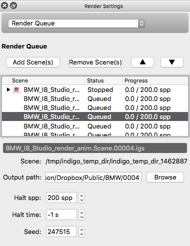
Render Queue
A Render Queue enables rendering a sequence of frames, Indigo scene files, with full control over the rendering process and halt settings for the different frames.
Creating a Render Queue
When exporting an animation from one of Indigo's 3D modelling package plugins, the Render Queue and an Indigo Queue file is created automatically.
When loading a scene from inside the Indigo GUI, only a single item is added to the render queue, however multiple scenes can be added using the Add Scene(s) button, with a halting condition (on rendering time, samples per pixel or both) to specify how long they should render for. To change halt conditions for multiple frames, simply shift click to select the desired frames, or use ctrl - A (cmd-A on Mac OS X) to select all of them, then change the values to your liking. When changing output paths for the rendered frames, you can use '%frame', which will be replaced with the frame index (0001, 0002, etc.).
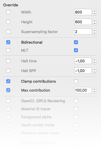
Overrides
As of version 4, Indigo has override capabilities for all render settings. This enables the user to change parameters like resolution, render method and clamping for all frames in an animation or sequence. To change a setting, use the controls on the right of the setting. To use the new setting for the other frames as well - simply tick the "Override" tick-box on the left.
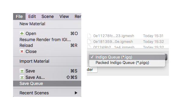
Indigo Queue and Packed Indigo Queue formats
To save an Render Queue, go to File -> Save Queue. You can then choose between an Indigo Queue (.igq) format and a Packed Indigo Queue format.
- The Indigo Queue option saves the Render Queue data by itself and doesn't include any scene data.
- The Packed Indigo Queue is a self-contained archive with everything needed to render a sequence of scenes, including all referenced scenes, models and textures etc and with paths made relative. It can be unzipped with compression programs such as 7-Zip. This is the preferred format for distributing Indigo animations.
Opening either of these files in Indigo will add the referenced scene files to the Render Queue window.
Render Settings
This section documents the render settings available in Indigo. Some of these settings may not be exposed directly, depending on which modelling package you're using.
Render mode
Specifies the render modes Indigo should use to render the scene.
If you are unsure which to use, bi-directional path tracing is recommended. See also the render mode guide.
Foreground alpha
Renders and outputs PNG or EXR images with an alpha channel. The background are rendered completely transparent, whereas reflections and absorption in glass will show up semi-transparently in the render as expected.
Clamp contributions
Contribution clamping basically works as a firefly filter.
If enabled, and the max contribution is low, it won't allow bright spots (fireflies) onto the render.
As the max contribution gets higher and higher, brighter and brighter spots are allowed. Max contribution of infinity corresponds to contribution clamping being disabled.
Please note that, since it is clamping bright spots, it introduces bias into the render. Because of this it will be off by default. However it's a useful tool for artists, to remove fireflies from their images in a simple and efficient way.
Halt time
The number of seconds for which Indigo should render, after which the rendering is halted.
Halt SPP
The number of samples per pixel (SPP) Indigo should render to, before rendering is halted.
Network rendering
If network rendering is enabled, other computers on the network will assist in rendering the scene.
Normally the master computer also contributes in this process, however with the working master option disabled only the connected slave nodes will contribute to the rendering (leaving more resources available on the master).
Save un-tone mapped EXR
An un-tone mapped EXR image is saved in the renders directory.
Save tone mapped EXR
A tone mapped EXR image is saved in the renders directory.
Save IGI
An un-tone mapped Indigo Image (.IGI) file is saved in the renders directory.
Image save period
How often, in seconds, the rendered image(s) will be saved to the renders directory.
Super sample factor
Super sampling helps to eliminate hard edges and fireflies in the render, at the cost of additional memory (RAM).
The amount of additional memory required to store the rendered image is proportional to the square of the super sample factor, i.e. for a factor of 2, 4x more memory is required, and for a factor of 3, 9x more memory is required. Note that this does not affect the size of the final image, and does not affect the rendering speed much (as long as the additional memory required is available).
Watermark
If this is enabled, an Indigo logo is displayed on the bottom-right corner of the output render. This behaviour cannot be changed in the Free version of Indigo.
Info overlay
If this is enabled, a line of text is drawn on the bottom of each render with various rendering statistics and the version of Indigo it was rendered with.
Aperture diffraction
Selects whether aperture diffraction should be used. Please see the aperture diffraction documentation for more information.
Render region
Specifies a subset of the image to be rendered; useful for quick previews in complex scenes.
Render alpha
A render mode that sets the pixel alpha (opacity) based on if the pixel is considered to be in the scene foreground or background.
This allows you to composite your rendered image onto another image (such as a photographed background) in an image editing application. See Foreground Alpha.
Lens shift
Normally the lens is located in front of the middle of the sensor, however lens shifting allows you to move it. This is used to compensate for perspective effects when rendering with a relatively wide field of view.
Advanced render settings
Typically users will not have to change any of these settings. Changing these from their defaults can lead to unexpected results and we recommended leaving them at their defaults.
MNCR
MNCR stands for Max Number of Consecutive Rejections, a parameter used in the MLT rendering modes. A lower number can reduce "fireflies", but will introduce some bias into the render.
Auto choose num threads
Automatically chooses all available CPU cores for rendering. Turn this off to manually specify number of threads to use for rendering, in conjunction with the "num threads" option below.
Num threads
Define the number of threads for Indigo to render with.
Logging
If true, a log from the console output is written to log.txt in the current working directory.
Cache trees
If true, k-D trees and BVH data structures are saved to disk after construction, in the tree_cache directory. If the
Splat filter
Controls the filter used for splatting contributions to the image buffer. Either "fastbox" or "radial" are recommended; radial produces slightly higher quality images, but is blurry when used with a super-sampling factor of 1 (a factor of 2 or higher avoids this problem and delivers very high image quality).
Downsize filter
Controls the filter used for downsizing super-sampled images. Only used when super sample factor is greater than 1. The same filters used for splatting can be used for the downsize filter, with a few extra options (please consult the technical reference for more information).
Camera
Indigo implements a physically-based camera model which automatically simulates real-world phenomena such as depth of field (often abbreviated as DoF), vignetting and aperture diffraction.
This is a crucial component for Indigo's "virtual photography" paradigm, as it allows the user to use familiar settings from their camera in producing realistic renderings of their 3D scenes.
Aperture radius
Defines the radius of the camera aperture.
A smaller aperture radius corresponds to a higher f-number. For more information on this relationship please see the excellent Wikipedia page on f-numbers.
Focus distance
The distance in front of the camera at which objects will be in focus.

Aspect ratio
Should be set to the image width divided by the image height.
Sensor width
Width of the sensor element of the camera. A reasonable default is 0.036 (36mm). Determines the field of view (often abbreviated as FoV), together with the lens sensor distance.
Lens sensor distance
Distance from the camera sensor to the camera lens. A reasonable default is 0.02 (20mm).
White balance
Sets the white balance of the camera. See White Balance.
Exposure duration
Sets the duration for which the camera's aperture is open. The longer the exposure duration, the brighter the image registered by the sensor.
Autofocus
When this option is enabled Indigo will perform an autofocus adjustment before rendering, automatically adjusting the focal distance based on the distance of objects in front of the camera.
Obstacle map
An obstacle map texture is used when calculating the diffraction though the camera aperture, to change the way the aperture diffraction appears.
Aperture shape
This allows a particular shape of camera aperture to be specified.
The allowable shapes are "circular", "generated" or "image". A preview of the final aperture shape will be saved in Indigo's working directory as "aperture_preview.png". An image aperture shape must be in PNG format and square with power-of-two dimensions of at least 512 x 512. The image is interpreted as a grey-scale image with the white portions being transparent and black being solid.
For further information and example images please see the aperture diffraction sub-section.
Aperture diffraction
Aperture diffraction allows the simulation of light diffraction through the camera aperture. Such diffraction creates a distinct "bloom" or glare effect around bright light sources in the image. The shape of the glare effect is determined by the shape of the aperture.
You can enable or disable aperture diffraction via the "Enable aperture diffraction" checkbox in the imaging section of the render settings view.
Post-process aperture diffraction dramatically increases the amount of memory (RAM) used, and the time taken to update the displayed image.
The following images illustrate the effect of aperture diffraction with various aperture shapes:

A simple render of the sun, without aperture diffraction enabled.

Aperture diffraction with a circular aperture.

Aperture diffraction with a 6-blade generated aperture.

Aperture diffraction with an 8-blade generated aperture.
Camera types
In addition to the normal thin-lens camera model, Indigo supports two additional camera types: orthogonal/parallel, and spherical.
Please note that these additional camera types are professional visualisation features and are only available in Indigo Renderer, and not Indigo RT.
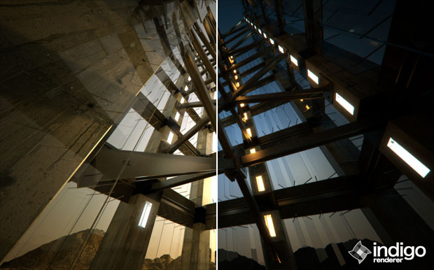
Thin-lens perspective camera
This is the default camera mode, with many familiar settings from standard photography. For more information please see the parent Camera page.
Concrete House scene by Axel Ritter (Impulse Arts)
Orthogonal/parallel projection camera
In this mode, there is no foreshortening due to perspective, i.e. objects far away appear the same size as those near to the camera. This is commonly used in architectural visualisation for building plans.
Please note that since there is no perspective in this camera mode, the sensor width needs to be very large in order to be able to image large objects; this can lead to somewhat implausible (though not unphysical!) circumstances in which you have building-sized sensors.
For more information please see the SkIndigo orthographic camera tutorial.

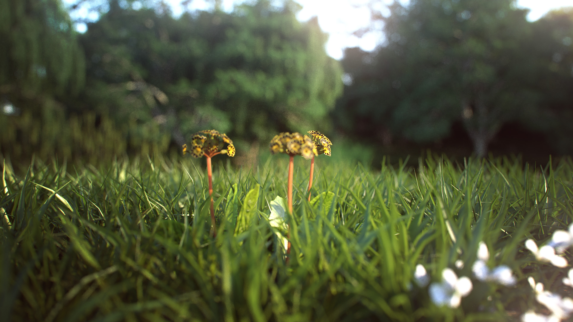
Garden Lobby scene by Tom Svilans (StompinTom)
Spherical projection camera
The spherical projection camera renders a complete 360 degree view at once, which is useful for making environment map renders (for example to use as High Dynamic Range images for illuminating other scenes). It can also be used to render images for 360 degree panorama viewing applications.
Because spherical maps cover twice as many degrees in longitude as latitude, it is recommended to make your spherical renders with aspect ratio 2:1 in X and Y.
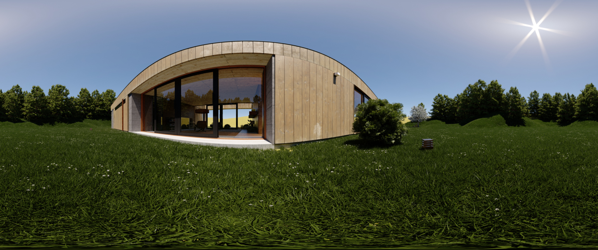
Weekend House scene by Axel Ritter (Impulse Arts)
Tone mapping
Tone mapping changes the brightness and contrast of your image. It can be done at any stage during the render process. Changes to tone mapping will be applied immediately to the rendered image. Tone mapping is non-destructive, so you can play around with the different tone mapping settings without permanently effecting the rendered image. You may want to tone map your image using different settings, and press Save Image to save out several different images.
How it works: Indigo creates a high dynamic range (HDR) image as it renders, and during the tone mapping process this will be converted to a low dynamic range red, green and blue image that can be displayed on your computer monitor. When subsequently saving the image, the user can choose to either save the tone mapped image in JPG, PNG, TIFF or EXR format. Indigo also supports saving of the un-tone mapped HDR image in EXR format for external tone mapping.
Tone mapping method comparisons
Indigo has four different tone mapping techniques that you can choose from: Reinhard, Linear, Camera and Filmic. Here are some comparisons of the different methods, and their strengths and weaknesses, using example scenes from Zalevskiy and Zom-B respectively.
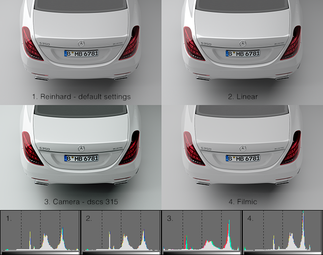
Note how the Camera tone mapping method gives the image a more photographic look with higher contrast and a slight colour tint.
Reinhard is the simplest to use, but once mastered, camera tone mapping can give a nice artistic feel to the renders.
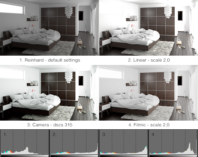
The Filmic tone mapper does a good job with achieving a bright look without burning out the whites.
Linear
The simplest tone mapping method, linear depends on just a single number. Every pixel in the HDR image will be multiplied by this number.
Reinhard
Reinhard is a method based on a paper by Reinhard, Stark, Shirley and Ferwerda from the University of Utah. It is an easy to use tone mapping technique because it automatically adjusts to the amount of light in the scene. It can be tricky to get linear or camera tone mapping to look balanced in scenes where there is an extremely bright light source – the Reinhard method is a good choice for scenes like this.
The default Reinhard settings of prescale=6, postscale=1, burn=2 will give good results for most renders. If you want to adjust the Reinhard method, below is an approximate description of each parameter.
| Prescale | Similar to a contrast control, works by increasing the amount of light in the HDR buffer. |
| Postscale | Works like a brightness control, increases the absolute brightness of the image after it has been tone mapped. |
| Burn | Specifies the brightness that will be mapped to full white in the final image. Can be thought of as gamma control. |
Camera
Camera tone mapping simulates the working of a photographer's camera. You adjust the exposure and ISO settings as you would in a real camera to modify the tone mapping.
The parameters you modify are:
| ISO | The ISO number represents the speed of film that is used. The higher the ISO number, the more light will be collected in the HDR Image. In low light situations, a fast film should be used, such as ISO 1600, and in bright lighting situations, a slow film can be used, such as ISO 100. |
| EV | The exposure value can range from -20 to +20 and represents a correction factor that is applied to the collected light. The higher the EV, the brighter the final image will be. Increasing the EV by one will make the image twice as bright. |
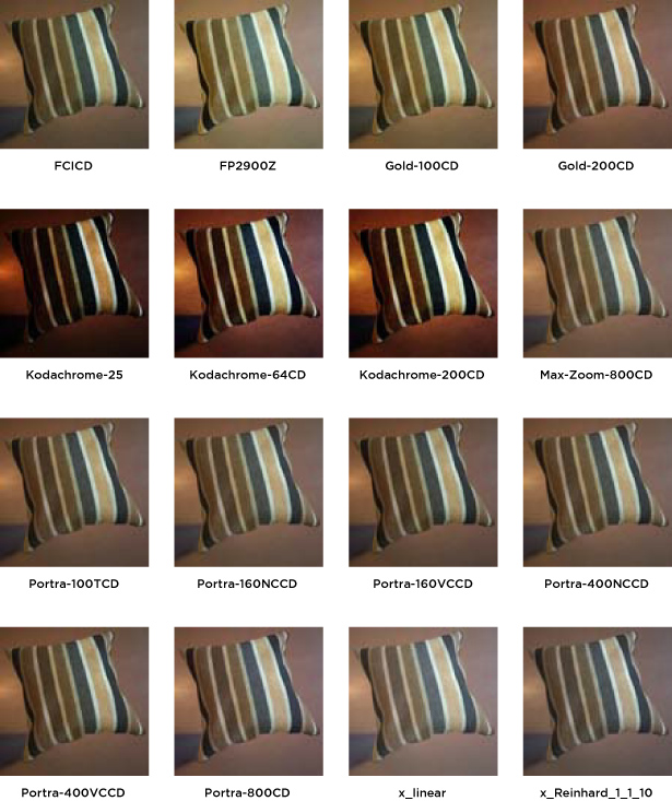
The final parameter is the response function. This specifies the type of film or digital camera to emulate. Different films and cameras emphasise different colours. The response functions are taken from real cameras – for example the images below use Ektachrome 100CD film which is famous for being used by National Geographic in their older photos.
A good default for sunny well-lit scenes is an ISO of 200 and an EV of -5.0.
Here are previews of each of the Camera Response Functions

|

|
|
| Page 1 | Page 2 | Page 3 |
Filmic
Like Linear, this tone mapper has only one control, scale, but it responds quite differently compared to Linear with significantly less contrast at high scale values. This makes it particularly suitable for creating bright images while (to an extent) preventing highlights to burn out.
Colour correction
The Imaging window in Indigo features two controls for simple colour correction: White Point, and Colour Curves.
White Point
This control adjusts the white point of the image via chromaticity coordinates x and y. There are a number of presets to choose from, with the option to edit the white point completely manually.
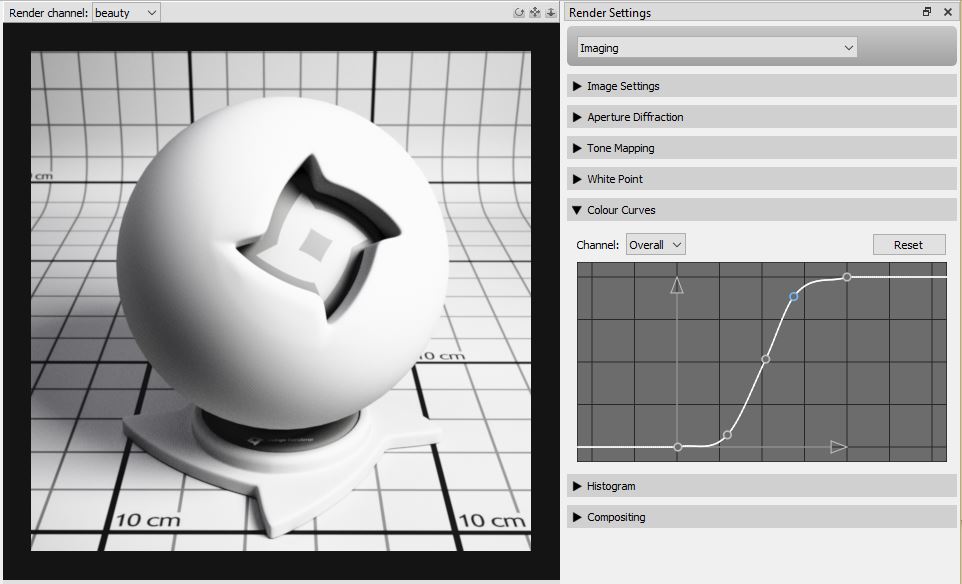
Colour Curves
Colour curves offer great control over tone and colour, right inside Indigo. There are curves for each RGB channel, as well as an Overall curve for control of overall brightness and contrast.
For each colour curve, the x coordinate (e.g. distance along the horizontal axis to the right) is the input value, e.g. how bright a pixel value is before it is transformed by the colour curve. The y coodinate (e.g. distance along the vertical axis upwards) is the output value, e.g. how bright a pixel value will be after it is transformed by the colour curve.
In this example image we are using the colour curve to generate more contrast in the image - in particular to make the blacks blacker and to saturate the brighter grey values towards white. This is achieved by using an S-shaped curve.
Render Mode Guide
The different render modes in Indigo each have their own strengths and weaknesses. Different render modes perform differently on different scenes - some render modes will produce less noise, and some render modes will produce more. Since Indigo is an unbiased renderer, all render modes will eventually produce the same resulting render however.
See the Render mode description page for more information on the various render modes.
In this section we will demonstrate the effect different render modes have on a couple of scenes. All images have been rendered for two minutes on a single computer.
The first scene shown here is an 'easy' scene: although there is a small light source, all materials are diffuse.
All render modes perform adequately on this scene, although the non-MLT modes (path tracing and bidirectional path tracing) perform better than the MLT modes.
This shows that MLT is not helpful on 'easy' scenes.
Path tracing render mode

Bidirectional path tracing

Path tracing with MLT

Bidirectional path tracing with MLT
The second scene shown here is the same scene as before, except that the diffuse material on the sphere has been replaced with a specular material. The combination of a small, bright, light source and a specular material make this scene a 'hard' scene.
The path tracing render mode struggles, producing 'fireflies' (white dots) over the image.
(These white dots are not errors, they are just 'noise' in the image, that will go away after a long enough render time)
Path tracing render mode
The bidirectional path tracing mode does much better. There are still some fireflies on the sphere. These are from the notoriously difficult 'specular-diffuse-specular' paths that are a problem for unbiased renderers.
Bidirectional path tracing
Path tracing with MLT 'smears-out' the fireflies produced with the path tracing render mode. However the result is still not great.
Path tracing with MLT
Bidirectional path tracing with MLT is the most robust render mode in Indigo, as it performs adequately even in 'hard' scenes such as this one. There are still some smudges / splotches in this image, but they will smooth out after longer rendering.
Bidirectional path tracing with MLT
Render mode description
Indigo is a ray tracer, which means that it renders scenes by firing out rays and letting them bounce around a scene to form ray paths. Different render modes control the way ray paths are constructed. Different render modes have different strengths and weaknesses for different kinds of scenes.
The main render modes are:
- Path tracing
- Bidirectional path tracing
- Path tracing with Metropolis Light Transport (MLT)
- Bidirectional path tracing with MLT
Generally, bidirectional path tracing should be used as it is the best all-round solution.
Metropolis light transport (MLT) can help rendering speeds in tricky scenes, such as scenes with small lights and glass panes, or sunlight reflected off glass or polished surfaces. See this page for more information about MLT.
Here is a diagram describing what they do:
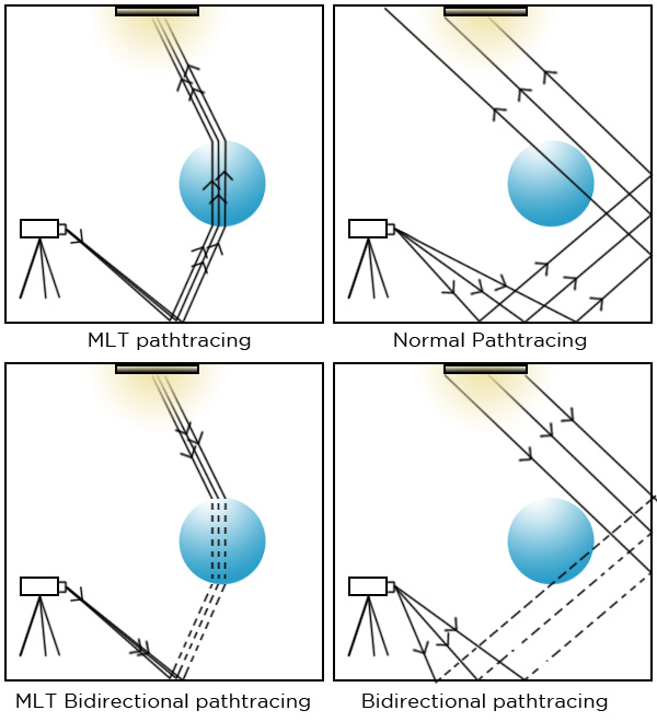
| Path tracing | Rays are fired from the camera, bouncing around the scene until they hit a light. |
| Bidirectional path tracing | Rays are fired from both the camera and light sources. They are then joined together to create many complete light paths. |
| Path tracing with MLT | Rays are fired from the camera, bouncing around the scene until they hit a light. When a successful light-carrying path is found, another is fired off on a similar direction. Gives good results for caustics. |
| Bidirectional path tracing with MLT | Rays are fired from both the camera and the lights, then connected to create many paths. When a successful light-carrying path is found, another is fired off on a similar direction. Gives good results for caustics and "difficult" scenes generally. |
There are also other, more specialised, rendering modes available for use in post-production:
 |
Shadows Only shadow catcher materials are rendered to an alpha layer, ready for compositing. Shadows render mode is Indigo Renderer only and is not available in Indigo RT. |
Material database
The online material database is a shared repository where users can view, download and share Indigo materials. These are distributed as either .IGM (Indigo Material) or .PIGM (Packed Indigo Material) files, the latter being preferred since it automatically packages all required textures.
Tutorials
Loading a material into the Indigo Material Editor
The first step is to download the material. To do this, click on the material thumbnail to go the material information page, for example http://www.indigorenderer.com/materials/materials/11.
Then click the download button above the material image. This will save an IGM or PIGM file to your computer.
Now click on the downloaded IGM or PIGM file. This should load the material into the Indigo Material editor and start rendering a preview of it.
Uploading a material to the database
The Upload Material button in the toolbar will upload the material applied to the preview object together with the currently rendered preview image. The preview must be sufficiently clean (at least 200 samples per pixel) otherwise the upload will not succeed.
An alternative way to upload materias is through the Indigo website by hovering over Materials in the section bar, then clicking Upload a material.
Materials
Accurately modelling the appearance of materials in a scene is crucial to obtaining a realistic rendered image. Indigo features a number of different material types, each customisable with various attributes, allowing great flexibility in material creation.
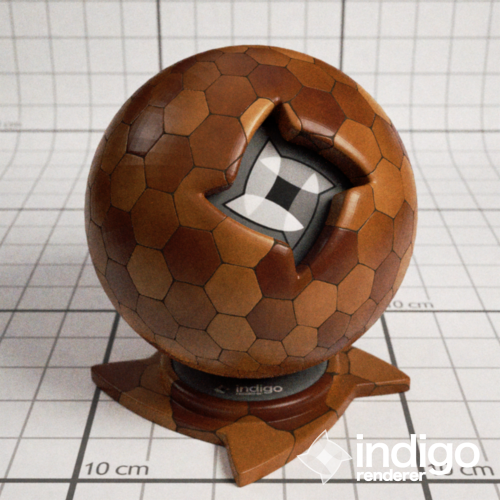
The material previews have been rendered in the main Indigo application (File -> New Material) using the default material ball scene.
Material Attributes
Indigo materials can have a number of attributes or parameters to control their appearance. Some of these are relatively common and simple, such as the Albedo parameter, however others such as Absorption Layer Transmittance are particular to a material type and warrant a detailed explanation.
Many of the parameters can be given either as a constant, a texture, or an ISL shader.
Albedo
Albedo can be thought of as a basic "reflectivity colour" for a material.
For example, if a material has an RGB albedo with each component set to 0.0, it will be completely black and reflect no light; with each component set to 1.0, light would never lose energy reflecting off the material, which is physically unrealistic.
A comparison of various albedo values found in nature is available on Wikipedia.
An example diffuse material with a green albedo.
Materials which have an albedo attribute:
Bump
Bump mapping gives the illusion of highly detailed surface without actually creating more geometry; in other words, it's a shading effect which gives a good approximation to more a detailed surface.
When specifying a texture map, the texture scale (B value) tells Indigo how far the distance is from full black to full white in metres. Since bump mapping is only intended to simulate small surface features, this value will be quite small since it is specified in metres, usually on the order of about 0.002.
See the Texture Maps section for information on texture attributes.
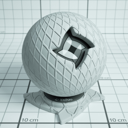
An example material with a grating texture used as a bump map.
Materials which have a bump attribute:
Diffuse
Phong
Specular
Oren-Nayar
Glossy Transparent
Displacement
Unlike bump mapping, which is a shading effect and does not create actual geometry, displacement mapping correctly generates new geometry from a base mesh and specified displacement map, by displacing the mesh vertices along their normals according to the displacement map.
This ensures that object silhouettes are correctly rendered, and is recommended for large displacements where bump mapping would look unrealistic; even mountain ranges can be efficiently created with this technique.
A constant setting displaces the entire mesh evenly by the defined amount. A texture map displaces the vertices based on values in a grey-scale image.
See the Texture Maps section for information on texture attributes.
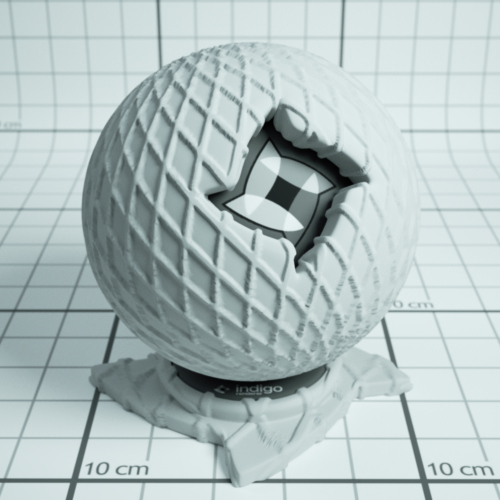
An example material a grating texture displacement map.
Materials which have a displacement attribute:
Diffuse
Phong
Specular
Oren-Nayar
Glossy Transparent
Diffuse Transmitter
Roughness
The roughness parameter controls the roughness of the surface, with lower roughnesses corresponding to a smoother, more polished surface with mirror-like reflections.
The roughness varies from zero to one, and it can be set using a texture or a shader.
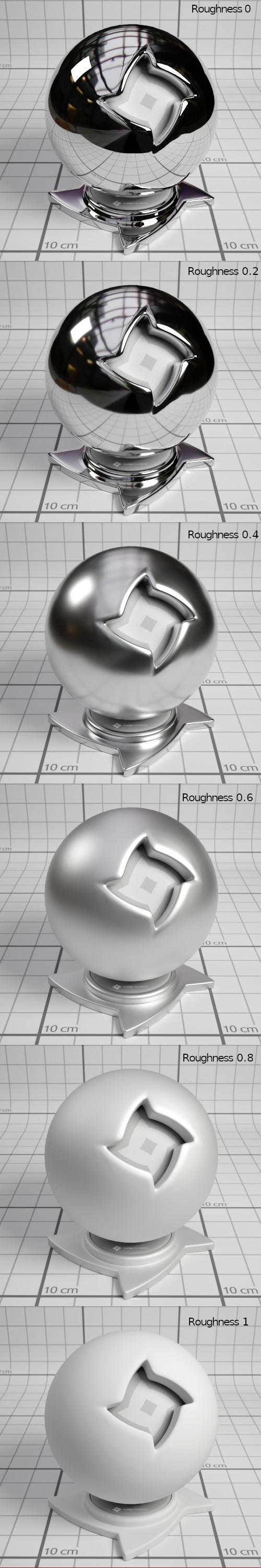
Example of Phong materials with different roughnesses.
Materials which have a roughness attribute:
Phong
Glossy Transparent
Coating
Double-sided Thin
Base Emission
This parameter specifies the base amount of light a material emits (in units of Lumens), which can be modulated using the Emission parameter.
This is used to create light sources.

An example of a 1500 Kelvin blackbody emitter.
| RGB: | Light based on colour and brightness. |
| Uniform: | A white light with intensity based on value given. |
| Blackbody: | Light is based on the temperature. Measured in Kelvin. |
| Peak: | Defines a band of wavelengths in which the material emits light. |
| Tabulated: | The emission spectrum is specified at regular wavelength intervals, which is useful for entering lab-measured data when a very controlled simulation is required. |
Materials which have a base emission attribute:
Diffuse
Phong
Specular
Oren-Nayar
Glossy Transparent
Diffuse Transmitter
Emission
The emission parameter multiplies the Base Emission to produce effects such as TV screens, where the brightness varies over the surface of the screen.
An emission scale parameter is available to scale the emission of the material by a given amount. Various photometric units are available.
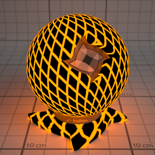
An example material with a 1500 Kelvin blackbody emitter, modulated by a grating texture.
Materials which have an emission attribute:
Diffuse
Phong
Specular
Oren-Nayar
Glossy Transparent
Diffuse Transmitter
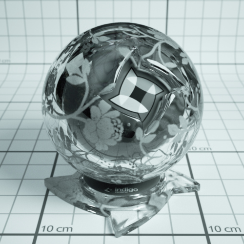
Absorption Layer Transmittance
Absorption Layer Transmittance refers to the absorption of light at the transmitting surface by a given "layer", which allows further control over how specular materials appear without changing the medium's absorption properties (which is what usually creates the perceived colour).
This can be useful for producing a stained glass window effect for example.
An example material with a grating texture used as an absorption layer.
Materials which have an absorption layer attribute:
Specular
Glossy Transparent
Layer
Light layers enable a rendered image to be split into additive "layers", in which each layer holds some contribution to the final rendered image.
How much a layer contributes to the final image can be adjusted interactively while rendering without restarting the process, and even after the render is completed, allowing for great flexibility in adjusting the lighting balance without having to do a lot of extra rendering. See Light Layers for more information on this subject.
The material's layer parameter specifies which light layer the (presumably light-emitting) material's contribution is added to.
Materials with attribute:
Diffuse
Phong
Specular
Oren-Nayar
Glossy Transparent
Diffuse Transmitter
Material Types
This section covers the various material types available in Indigo.
There are also video tutorials available for editing materials within Indigo, which include explanations of the material types, available here.
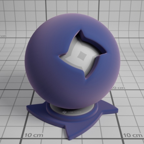
Diffuse
Diffuse materials are used for rough or "matte" surfaces which don't have a shiny appearance, such as paper or matte wall paint.

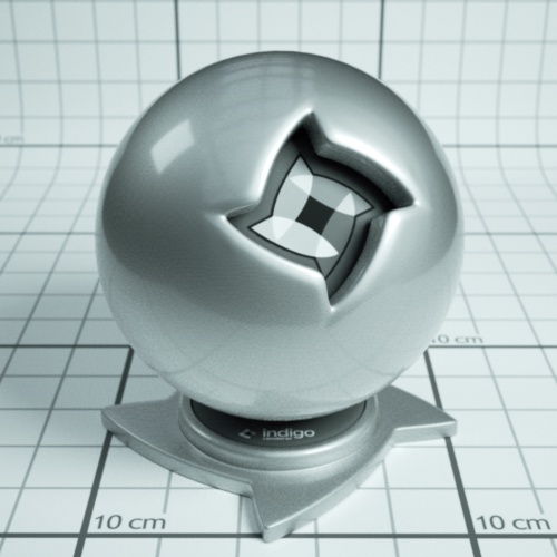
Phong
The Phong material is a generalisation of the Diffuse material type, adding a glossy coating on top of the diffuse base (or "substrate"). The influence of this coating is controlled by its index of refraction (IOR), with higher values corresponding to a stronger specular reflection. (the default IOR is 1.5)
It is commonly used for materials such as polished wooden floors, car paints (when multiple Phong materials are blended together) and metals.
Metals in particular can be represented using either the "specular reflectivity" option (which allows a specular colour to be defined for the material), or via measured material data (referred to as NK data).

IOR (Index Of Refraction): Controls the influence of the glossy coating; higher values produce a stronger specular reflection. The IOR should be set to the real-world value for the material, if available.
For example, the IOR of plastics is around 1.5 to 1.6.
Oil paint binder has an IOR of around 1.5.

Phong material with IOR 1.2

Phong material with IOR 1.5

Phong material with IOR 2.5
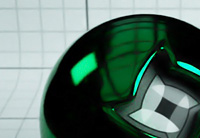
NK data: The Indigo distribution comes with a set of lab-measured data for various metals. If one of these data sets is selected, the diffuse colour and specular reflectivity colour attributes are ignored.
Specular reflectivity colour: When not using NK data, this allows you to set a basic colour for the metal; this is useful for uncommonly coloured metals such as Christmas decorations.
 |
 |
 |
| Green specular colour | Au (gold) NK dataset | Al (aluminium) NK dataset |
Attributes:
Albedo
Bump
Displacement
Exponent
Base Emission
Emission
Layer
Specular
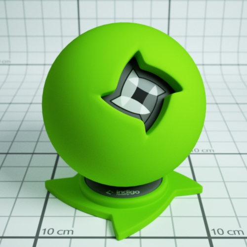
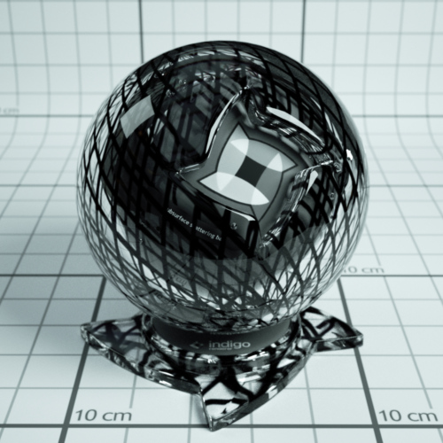
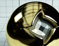
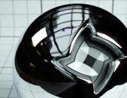
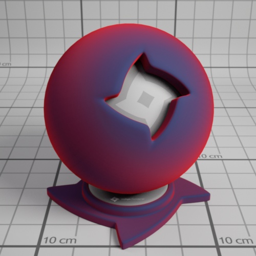
Specular materials are idealised materials which refract and/or reflect as in classical optics for perfectly smooth or flat surfaces (e.g. mirror-like reflection).
A specular material can either transmit light, as is the case with glass and water for example, or not as is the case with metals. This behaviour is controlled by the material's "Transparent" attribute.
If a specular material transmits light, it will enter an internal medium whose properties define the appearance of the material (such as green glass, which has absorption mainly in the red and blue parts of the spectrum). For more information on this please see the correct glass modelling tutorial.
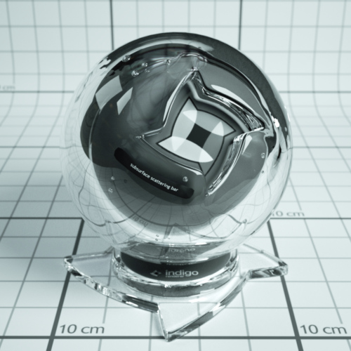
Transparent: If enabled, it allows light to pass through the material. Otherwise only reflected light is simulated.
Attributes:
Albedo
Bump
Displacement
Base Emission
Emission
Absorption Layer Transmittance
Layer
Internal Medium
Oren-Nayar
Oren-Nayar materials are another generalisation of the basic diffuse material type, except unlike Phong which generalises to shiny surfaces, Oren-Nayar generalises to rougher materials.
The appearance is quite similar to diffuse materials, but with less darkening at grazing angles; this makes it suitable for modelling very rough or porous surfaces such as clay or the moon's surface.

Sigma: Controls the roughness of the material. A higher sigma gives a rougher material with more back-scattering. The default sigma value is 0.3, and values higher than 0.5 primarily cause energy loss / darkening due to strong inter-reflection. A value of 0.0 corresponds exactly to diffuse reflection.
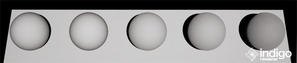
From left to right: Diffuse material, then Oren-Nayar with sigma values 0.0, 0.2, 0.5, 1.0.
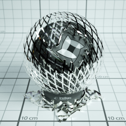
Glossy Transparent
The glossy transparent material is a generalisation of the specular material, to allow non-perfect (i.e. rough) reflection and refraction, via an exponent parameter as with the Phong material.
It is commonly used for materials such frosted glass or even human skin (with a low exponent value).
![]()
Attributes:
Exponent
Internal Medium
Absorption Layer Transmittance
Bump
Displacement
Base Emission
Emission
Layer
Diffuse Transmitter
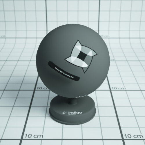
The diffuse transmitter material simulates a very rough transmitting material, which reflects no light back outwards. For this reason it is normally blended with a normal diffuse material to model surfaces such as curtains or lampshades.
It is meant to be used on single-layer geometry, and although it does not have an associated internal medium by default, it is possible to use one.
![]()
An example of the diffuse transmitter material on its own.
![]()
A blend between diffuse transmitter and normal diffuse materials to simulate the appearance of a curtain.
Attributes:
Albedo
Displacement
Base Emission
Emission
Layer
Blend
The blend material type isn't a material per se, rather it combines two sub-materials using blending factor.
This blending factor is a regular channel, and so can be constant, a texture or an ISL shader, allowing for great flexibility in material creation; a blend material can also use a blend as input, enabling so-called "shading trees" of arbitrary complexity.
Note that it's not possible to blend any combination of null and specular materials, except for the case where two specular materials with the same medium are being combined.
An example blend material from the material database, showing a blend between specular and diffuse materials.
Blend: Controls the amount of each material used. A value of 0 means only Material A is used, a value of 1 means only Material B is used, 0.5 implies a 50/50 blend, etc.
Step Blend: Instead of allowing partial blends, only one of Material A or Material B are selected, depending on whether the blending factor is below or above 0.5, respectively. This is recommended for "cut-out" clipping maps (such as for tree leaves), which produce less noise using this technique.
Exit Portal
When rendering interior scenes, one frequently encounters an efficiency problem where the "portals" through which light can enter the scene from outside (e.g. an open window) are relatively small, making it quite difficult to sample.
Exit portals can greatly improve rendering efficiency in these situations by marking important areas through which light can enter the scene, which Indigo will directly sample to produce valid light carrying paths.
Although it is a material type, exit portals don't have any particular appearance of their own, they simply provide an "open window" through which the background material is seen, and through which it can illuminate the scene.
For more information and example images, please see the SketchUp exit portal tutorial.
Requirements for exit portal usage:
- If any exit portals are present in the scene, then all openings must be covered by exit portals.
- The face normals must face into the interior of the scene.
- The exit portal material should only be applied to one side of a mesh (e.g. a cube), otherwise it will lose its effectiveness.
Coating
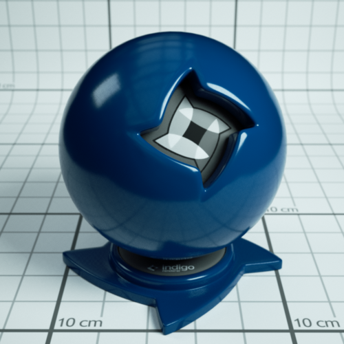
The coating material simulates a thin coating of some kind of material over another material. For example, you can create a thin coating of varnish over a metal material.
A coating material over a metal metal
The coating material can also simulate interference, which can give interesting effects when the thickness of the coating varies with position:
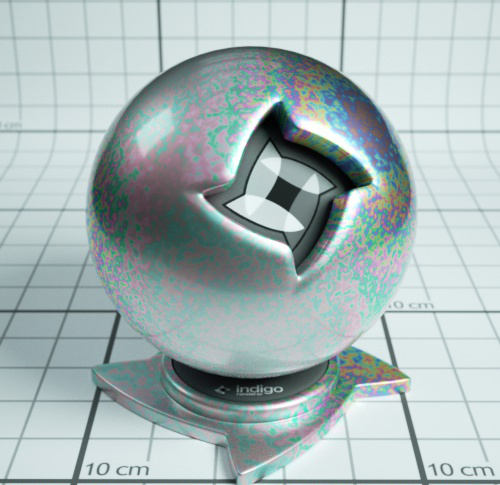
A coating material over a metal metal with interference enabled. Coating thickness is controlled with a shader.
Depending on the thickness of the coating, and how the thickness varies over the object (which can be controlled by a shader) you may get a kind of rainbow effect, or the material may just take on just a few colours:

400 nm thick coating showing colours from interference.
A coating can also absorb light, which will result in a tinted colour:

Coating with absorption over a metal material. The red colour comes from the absorption of non-red light as light passes through the coating layer.
Coating material attributes
Absorption
Controls the absorption of light as it travels through the coating layer.

Coating without absorption

Coating with absorption
Thickness
Controls the thickness of the coating layer. In the Indigo graphical user interface, the thickness is given in units of micrometres (μm), or millionths of a metre.
A thicker layer will have stronger absorption.

Coating with absorption, thickness of 100 μm.
Coating with absorption, thickness of 10000 μm.
Interference
If enabled, thin film interference is computed for the coating layer.
The result will be most noticable when the coating layer is on the order of 1 μm thick.

Coating without interference, thickness 0.6 μm.

Coating with interference, thickness 0.6 μm.
Double-Sided Thin
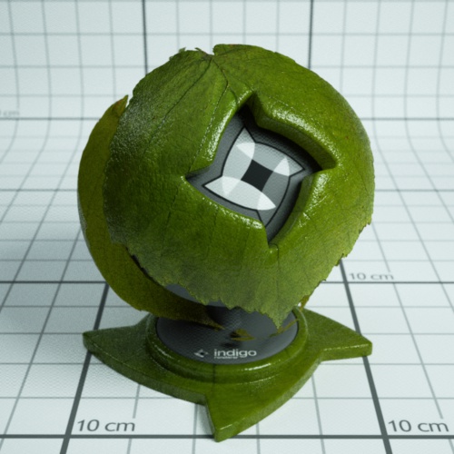
The double-sided thin material is useful for modelling thin objects, such as paper or plant leaves.
The double-sided thin material uses two 'child' materials: the front material and the back material, which are used for the front and back of the surface respectively. This means that you can make, for example, a leaf material where the front uses a different texture from the back.
It is also possible to specify the transmittance colour, which controls how light is absorbed and coloured as it passes through the object.

Render using double-sided thin material by Enslaver
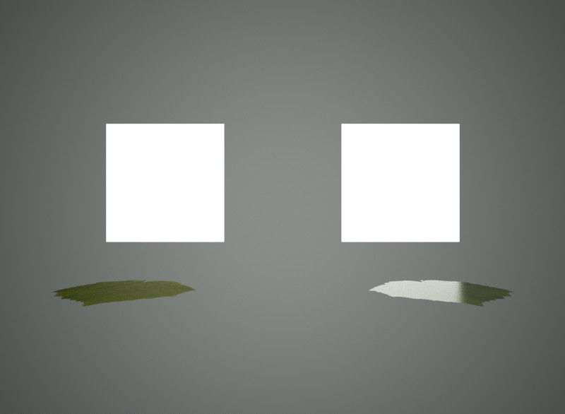
Leaf example
When the leaf is lit from the front, you can see that the leaf colour differs based on if the leaf is front or back side towards the camera: (The leaf on the right has the front/top side towards the camera) The light is behind the camera.
.jpg)
Leaf lit from front
When lit from the back, the leaf looks the same from both the front and the back. This is also what happens with a real leaf (try it!)
.jpg)
Leaf lit from back
The roughness (exponent) of the top can be varied independently of the roughness of the bottom of the leaf.
In this render the leaf on the right is frontside-up, on the left backside-up:
Leaf lit from top
Double-sided Thin Attributes
IOR: This is the index of refraction of the thin slab.
Front material: For light that is reflected diffusely back from the front surface, the front material controls the distribution of such light. Should be diffuse or Oren-Nayar. This material would be, for a leaf example, a diffuse material using the front-side albedo texture of your leaf.
Back material. For light that is reflected diffusely back from the back surface, the back material controls the distribution of such light. Should be diffuse or Oren-Nayar. This material would be, for a leaf example, a diffuse material using the back-side albedo texture of your leaf.
r_f: this is the fraction of light that enters the slab that is reflected back to the side it came from.
A good default value is 0.5
Transmittance: Some light scatters right through the slab and out the other side. The transmittance controls the absorption of such light. This is where you would use, for example, your transmittance map of a leaf.
Front Fresnel scale: A factor that controls the intensity of the specular scattering off the front interface of the slab. Default value is 1.
Back Fresnel scale: A factor that controls the intensity of the specular scattering off the back interface of the slab. Default value is 1.
Front Roughness: Controls the roughness of the front interface of the slab.
Back Roughness: Controls the roughness of the back interface of the slab.
Fabric
The Fabric material is useful for modelling textiles, such as cotton, wool, velvet etc. It is similar to a diffuse material except the edges of the material appear a different colour. This simulates forwards and backscattering due to small hair fibres.
Fabric Material Attributes
Colour: This is the main colour of the fabric. As usual it can be a constant colour, a texture, or a shader.
Roughness: This controls the roughness of the surface. A rougher surface will have a wider sheen 'highlight'.

Roughness = 0.1
Roughness = 0.9
Sheen colour. This is the colour of the sheen. The sheen is generally backscattered light, seen around edges of the objects.
For example, this fabric material uses a red sheen colour:
Sheen weight: This is the strength of the sheen reflection.
Sheen weight = 0.1
Sheen weight = 0.9
Null
The null material is not a normal material type (like the exit portal material), but rather indicates that light should pass straight through it, unaffected in brightness and direction.
This on its own is not very helpful, however when combined with the blend material type it becomes very useful for making "cut-outs" such as leaf edges, which would otherwise highly complex geometry.
An example of the null material on its own.
An example of the null material blended with a Phong metal, using a grating texture as blend map.
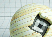
Texture Maps
Texture maps are a standard way of adding fine surface detail without adding more geometry. Indigo supports texture maps in many file formats, which are listed here.

An example Phong material with a wood texture applied.
Supported texture formats:
| JPEG | .JPG .JPEG | Greyscale, RGB and CMYK are supported. |
| PNG | .PNG | Greyscale, greyscale with alpha, RGB and RGBA are supported. 8 bits per channel and 16 bits per channel supported. |
| Truevision Targa | .TGA | Greyscale (8 bits per pixel) and RGB (24 bits per pixel) are supported. |
| Windows Bitmap | .BMP | Greyscale (8 bits per pixel) and RGB (24 bits per pixel) are supported. Compressed BMP files are not supported. |
| OpenEXR | .EXR | 16 bits per channel and 32 bits per channel are supported. |
| TIFF | .TIF .TIFF | Greyscale, RGB, RGBA are supported. 8 bits per channel and 16 bits per channel supported. |
| GIF | .GIF | Supported. Gif animation is not supported. |
| RGBE | .HDR | Supported. |
Additional options:
| UV set index | Index of the set of uv coordinates used for texture maps. Usually generated by your 3D modelling package. |
| Path | Path to the texture map on disk. The path must either be absolute, or relative to the scene's working directory. |
| Gamma (exponent) | Used for converting non-linear RGB values (e.g. sRGB) to linear intensity values. A typical value is 2.2, corresponding to the sRGB standard. |
ABC values / texture adjustments
Often you'll want to change a texture's brightness or contrast in the rendered image, without having to modify the texture map itself.
During rendering, Indigo modifies the source texture data according to a quadratic formula with 3 parameters, A, B and C:
y = ax² + bx + c
x is the input value from the texture map, and y is the output value.
As a quick example for how this equation works: If we use A = 0, B = 1, C = 0 then the value is completely unchanged; this is therefore also the default.
A value – Quadratic
The A value scales the contribution of the quadratic (x²) term. This is typically not used, however it can be useful to adjust the contrast of a texture, with a value greater than 0, and/or a negative C value.
B value - Scale/Multiplier
Texture Scale (B value) of 2.
The B value scales the contribution of the linear (x) term. This is typically used to adjust the overall brightness (for example to reduce the maximum albedo of a texture, using a value of 0.8 or so), and can also be useful to adjust the contrast of a texture, with a value greater than 1, and/or a negative C value.
C value – Base/Constant

Texture constant (C value) of 0.2.
The C value is always added, regardless of the input texture amount; it therefore acts as a base or "floor" value. So for example if you have a completely black texture, and a C value of 0.5, it would appear as 50% grey.
Internal Medium
A (transmission) medium defines the properties of the matter through which light travels, when it is refracted at a material interface.
For example, a green glass medium will specify moderate absorption in the red and blue parts of the spectrum, so as to leave behind mainly green light; clear blue water will specify a small amount of absorption in the red and green parts of the spectrum so as to leave behind mainly blue light. If the medium contains many small particles, such as milk, then it will also specify other properties such as the scattering coefficient, etc.
- The object has to be a closed volume. This means it cannot have any holes leading to the interior of the mesh.
- All mesh faces must be facing outwards. Check the face 'normals'.
Precedence: Precedence is used to determine which medium is considered to occupy a volume when two or more media occupy the volume. The medium with the highest precedence value is considered to occupy the medium, 'displacing' the other media. The predefined and default scene medium, 'air', has precedence 1.
Basic
Typical values for glass and water lie in the range 0.003 – 0.01 (see http://en.wikipedia.org/wiki/Cauchy%27s_equation for some coefficients)
| IOR | Index of refraction. Should be >= 1. Glass has an IOR (index of refraction) of about 1.5, water about 1.33. The IOR of plastic varies, 1.5 would be a reasonable guess. |
| Cauchy B Coeff | Sets the 'b' coefficient in Cauchy's equation, which is used in Indigo to govern dispersive refraction. Units are micrometers squared. Setting to 0 disables dispersion. Note: the render can be slower to converge when dispersion is enabled, because each ray refracted through a dispersive medium can represent just one wavelength. So only set cauchy_b_coeff to other than 0 if you really want to see dispersion. |
| Absorption Coefficient Spectrum | Controls the rate at which light is absorbed as it passes through the medium. |
| Subsurface Scattering | Use this element to make the medium scatter light as it passes through it. |
| Scattering Coefficient Spectrum | Chooses the phase function used for the scattering. |
Phase Function
The phase function controls in which direction light is scattered, when a scattering event occurs.
| Uniform | Takes no parameters |
| Henyey Greenstein | The Henyey-Greenstein phase function can be forwards or backwards scattering, depending on the 'g' parameter. |
Dermis
| Hemoglobin Fraction | Controls the amount of hemoglobin present. Typical range: 0.001 – 0.1 |
Epidermis
Medium for simulating the outer layer of skin.
| Melanin Fraction | Typical range: 0 – 0.5 |
| Melanin Type Blend | Controls the amount of eumelanin relative to pheomelanim in the tissue. Typical range: 0 – 1 |
Material Database
The online material database is located at http://www.indigorenderer.com/materials/
There you are able to browse and download any of the user uploaded materials, and upload your own.
Please note that you cannot upload textures that you do not have the right to redistribute.
Indigo Shader Language
A fully procedural material made by galinette.
ISL stands for Indigo Shader Language. It's a functional language that allows you to write shaders for every channel in Indigo materials. With shaders you are not tied to the restrictions of textures any more: they are procedurally computed for every point on the surface.
Indigo Shader Language Beginner Tutorial
Indigo Shader Language Beginner Tutorial
This tutorial covers:
-What's ISL? And why should I use it?
-What's a functional language?
-How to define functions
-Which channel expects what function parameters an return value?
-What data-types are there?
-Functional, huh? Does that mean I have to use functions instead of operators?
-How to use a shader in a material?
-Going further
What's ISL? And why should I use it?
ISL stands for Indigo Shader Language. Its a functional language that allows you to write shaders for every channel in Indigo materials. With shaders you're not tied to the restrictions of textures any more because they are procedurally computed for every point on the surface (or in the volume, as of Indigo 2.4's ability to have volumetric shaders).
What's a functional language?
In functional language there are only functions that are used to compute something, no variables no loops (unless you write them as a function). By functions it means functions in the mathematical sense, it calculates something and returns the result. Lets have a look at this shader function: def doSomething(vec3 pos) real: noise(fbm(pos * 3.0, 8)) This is a function called 'doSomething', it has one parameter, a vector called 'pos' and it returns a real value. It uses two other functions, fbm() and noise().
Now what's happening here?
Like in a mathematical function you calculate the innermost parenthesis first. That means the vector 'pos' is multiplied by 3.0, then passed to the fbm() function which calculates a value of the type 'real', which is then passed to the function noise(), which calculates a 'real' value, which is the return value of the function 'def'. Pretty simple, isn't it?
How to define functions
Now, lets see how to define a function. A ISL function definition always starts with the keyword 'def', needs at least a name and a return value type, and it can also have function parameters: def name(parameters) return_value_type: [...actual function...] Although you can give your functions an any name you want the main function in a channel always has to have the name 'eval'. Which takes us directly to the next topic: different channels expect different parameters and return values!
Which channel expects what function parameters an return value?
There are three different channel types, wavelength dependent, wavelength independent and displacement. Wavelength dependent expects a vec3 as a return value, wavelength independent expects a real and displacement expects real and cannot use the position in world-space (vec3 pos) as a function parameter. Here's a table that illustrates all that: C
|
Channel |
Channel type |
Eval function expected |
|
Diffuse |
Wavelength dependent |
def eval(vec3 pos) vec3: |
|
Emission |
Wavelength dependent |
def eval(vec3 pos) vec3: |
|
Base Emission |
Wavelength dependent |
def eval(vec3 pos) vec3: |
|
Specular Reflectivity |
Wavelength dependent |
def eval(vec3 pos) vec3: |
|
Absorption Layer |
Wavelength dependent |
def eval(vec3 pos) vec3: |
|
Exponent |
Wavelength independent |
def eval(vec3 pos) real: |
|
Sigma |
Wavelength independent |
def eval(vec3 pos) real: |
|
Bump |
Displacement |
def eval() real: |
|
Displacement |
Displacement |
def eval() real: |
|
Blend |
Displacement |
def eval() real: |
What data-types are there?
First of all, its very important to know that ISL does not convert values implicitly, so if a function expects an integer, you have to make sure you give pass an integer value instead of a real.
-
real – floating point number
A real value always has to be written as a floating point number, for example 214.0.
-
int – whole numbers
Only whole numbers, like 20 or -1545.
-
vec3 – 3 component vector
There are two constructors for a vec3, vec3(real x) and vec3(real x, real y, real z). The first one applies the number passed to any of the 3 components and the second one sets each component separately. You can access the three components separately with the functions doti(), dotj() and dotk().
-
vec2 – 2 component vector
Like vec3, only just 2 components.
-
bool
A boolean value, true or false.
-
mat2x2 and mat3x3
2x2 and 3x3 matrix, I'm not going to talk about these right now.
Functional, huh? Does that mean I have to use functions instead of operators?
No, you don't have to use functions as operators, but you can, if you like to, are a hardcore mofo or just a little insane :) Operators are available for multiplication, division, addition and subtraction (*, /, + and -, would you believe it?) for every data-type that supports them, but the order of operands is important sometimes, for example: 0.333 * vec3(5.2) will not work since it expects the vec3 first. Vec3(5.2) * 0.333 works. The equivalent functions are called mul(), div(), add() and sub().
How to use a shader in a material?
Your exporter most likely has an option to use ISL shaders, also, you can use ISL in the Indigo Material Editor it allows you to use ISL shaders. And if you're hardcore, you can edit the .igs file generated by you exporter and insert your shaders manually, here's how you do it: Open the .igs file and look for a material. I'll just assume we found a phong material:
<material>
<name>phong_mat</name>
<phong>
<ior>1.466</ior>
<exponent>
<constant>800</constant>
</exponent>
<diffuse_albedo>
<constant>
<rgb>
<rgb>0.588235 0.588235 0.588235</rgb>
<gamma>2.2</gamma>
</rgb>
</constant>
</diffuse_albedo>
</phong>
</material>
What you have to do is, is to replace the <constant>...</constant> XML elements (and anything in between) in the diffuse_albedo channel with this:
<shader>
<shader>
<![CDATA[
#paste your shader in here, oh by the way: every line starting with # is a comment
)]]>
</shader>
</shader>
Then paste your shader in between '<![CDATA[' and ')]]>'.
Going further
For a complete list of all available functions, have a look at the ISL section in the 'Indigo Technical Reference.pdf' and the 'ISL_stdlib.txt' in the Indigo folder. Also, more ISL tutorials are coming!
Indigo Shader Language Tutorial
ISL stands for Indigo Shader Language, the language for creating procedural materials in Indigo. Since it's a functional language, it can be a bit tricky to create some patterns that are easy enough in an imperative language. For example, lets say you want to write a shader to make a polka-dot pattern. In an imperative language you might write some code like
def fillWithColour(background_colour):
	for(int x=0; x<W; ++x) {
		for(int y=0; y<H; ++y) {
			drawDot(x, y, dot_colour);
		}
	}
But in ISL, you can't do things this way. You have to write a function that returns the colour, and that depends only on the position and/or UV-coordinates of the current surface point being shaded, e, g:
def getColourForPoint(u, v):
	if( the point (u, v) is inside a dot ){
		return dot_colour
	} else {
		return background_colour
	}
This tutorial shows you how to use such a functional technique to create regularly repeating patterns, like polka-dots, with ISL.
Lets start by discussing the fract function.
As described in the Indigo Renderer Manual, fract takes a single real number, and returns a real number:
fract(x) = x - floor(x)
The useful thing about this function, is that it repeats regularly across the real number line, with period 1. We can use this function to create more complicated behaviour.
So lets say we want to create some stripes, such that they alternate in the U direction of the UV coordinates. Suppose we have a foreground and background colour.
Using the fract function above, we can can assign the foreground colour when fract(x) < C, and the background colour when fract(x) >= C, where C is some constant between 0 and 1. If C is 0.5, the stripes will have the same width as the background stripes.
Let's see how that looks in real ISL:
<material>
	<name>previewmaterial</name>
	<diffuse>
		<albedo>
			<shader><shader><![CDATA[
def eval(vec3 pos) vec3 :
	if(
		fract(doti(getTexCoords(0))) < 0.5,
		vec3(0.9, 0.0, 0.0), # Red
		vec3(0.2, 0.2, 0.2) # Dark Grey
	)
			]]></shader></shader>
		</albedo>
	</diffuse>
</material>
And the resulting render:

The shader with fract(x), so slowly repeating stripes.
In this example the foreground colour is red, and the background colour is dark grey. This example looks a bit weird because the stripes are large compared to the model. We can solve this problem by multiplying the UV coordinates by a number greater than one before we pass the value to fract, e.g we could use something like fract(10 * x)
The ISL is then:
def eval(vec3 pos) vec3 :
	if(
		fract(doti(getTexCoords(0)) * 10.0) < 0.5,
		vec3(0.9, 0.0, 0.0), # Red
		vec3(0.2, 0.2, 0.2) # Dark Grey
	)
And the resulting render is:

The shader with fract(10 * x) so more repeating stripes.
So, at this point in the tutorial, we have more-or-less solved the problem of how to create regularly-repeating patterns, at least with respect to the U coordinate (e.g. in one direction).
IES Lights
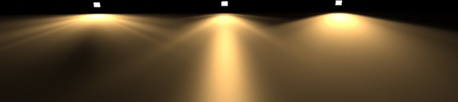
If an IES profile is selected, the distribution of emitted light is specified by the information in the IES profile. This is an easy way to get realistic emission profiles for a given light fixture, without creating a detailed model of the fixture.
Please note that only IES files with vertical angles below 90 degrees are currently supported.
See also the IES tutorial in the Techniques section of this manual.
Some freely available IES profiles are available to download from http://www.indigorenderer.com/dist/ies-profiles.zip
Mesh Settings
There are some settings that control how a triangle mesh is rendered in Indigo - in particular the subdivision and displacement settings. Please read on for details on these.
Instancing
Instancing is a way to replicate scene geometry or meshes without using much additional memory - each instanced object shares the original mesh data, however the material and placement in the scene can be different.
This is useful in many situations where there are multiple copies of the same mesh data (such as chairs around a table, or trees in a forest) to reduce the memory usage required for detailing an environment.
An excellent example is given below by forum user Godzilla:
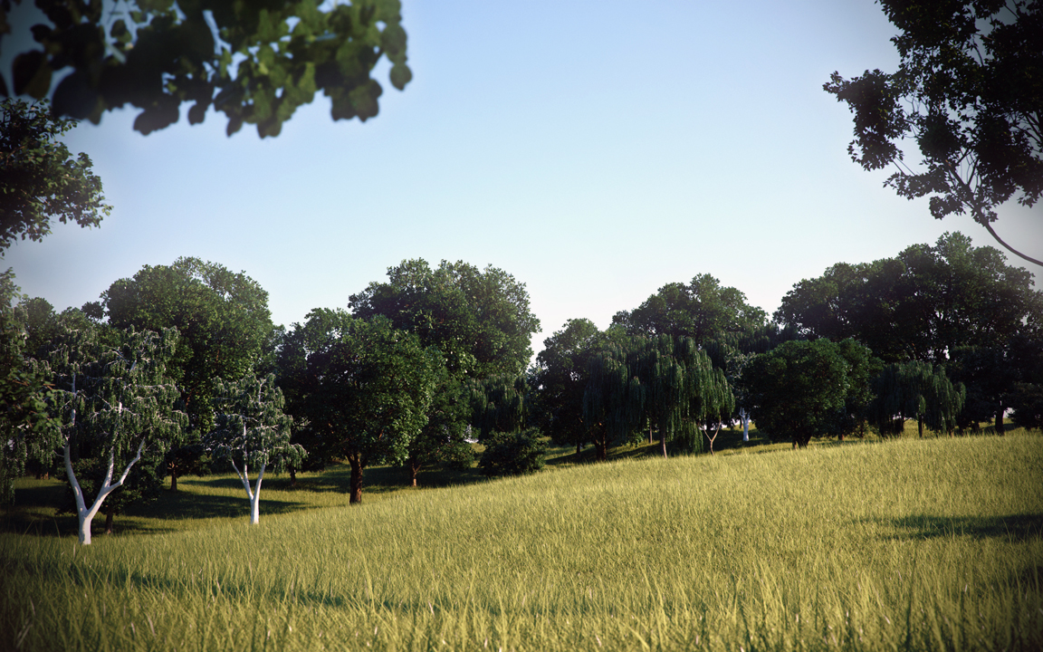
Image by Godzilla
Subdivision
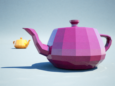 |
| Subdivison off |
 |
| Subdivison On |
Subdivision divides each triangle in the mesh into 4 new triangles, with each subdivision level increasing the number of triangles exponentially. Therefore a large mesh of, say, 1 million triangles becomes 4 million triangles when subdivided only once. When subdivided twice it becomes 16 million triangles, and when subdivided three times it becomes 64 million triangles.
Below are available settings:
| View Dependent | Subdivide only meshes visible by the camera |
| Max Subdivisions | How many times to subdivide the mesh. Polycount becomes exponentially larger with each subdivision level. |
| Curvature Threshold | Triangles will not be subdivided if their curvature is smaller than this threshold. |
| Pixel Threshold | Triangles will not be subdivided if they are smaller than this pixel threshold. |
Light Layers
Light layers allow you to separate contributions from different lights onto different "layers". Each layer can then be manipulated separately, even after the render has completed.
You can change the brightness of each layer, or change the overall colour of each layer, or even turn each layer off completely.
Enabling Light Layers
By default, all lights in an Indigo scene are assigned to Layer 0. This means that the HDR image will have only one layer – Layer 0. However, in the exporter for your 3D modelling program, you can change the layer that a light is assigned to. All contributions from that light will then be rendered onto that layer.
Each layer has a number of controls that you can manipulate in the Indigo GUI; please see the corresponding section in the Indigo interface section.